Every winter the Arctic sea ice spreads across an area larger than Europe, then partly melts back in summer. The models that project its future are getting it wrong, and not in the reassuring direction. A team from the University of Cambridge and the CIMAT research centre in Mexico has just shown this using a witness 6,000 years old. Their correction takes about a million square kilometres off the projections.
March 2026: the smallest maximum on record
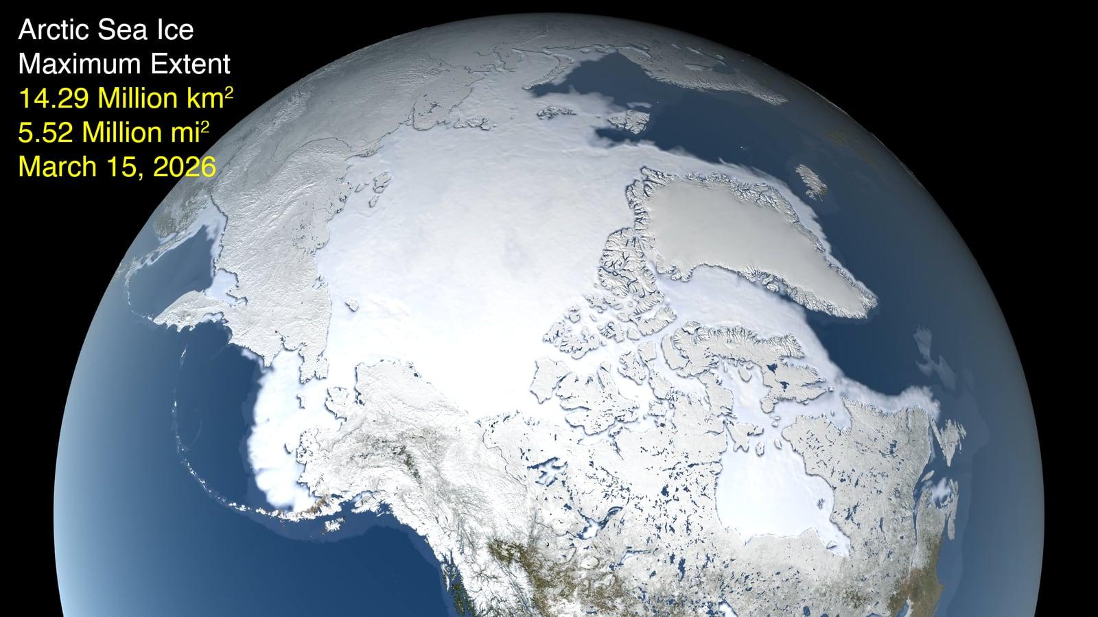
Start with the measurement, because it is recent and unambiguous. On March 15, 2026, Arctic sea ice reached its yearly maximum extent at 14.29 million km². That is the lowest maximum since satellite records began in 1978, statistically tied with the 14.31 million km² of 2025.
To make sense of the number, you need a baseline. The average maximum between 1981 and 2010 was 15.65 million km². Today's shortfall is therefore around 1.36 million km², roughly twice the area of Texas. Two records in a row do not prove much on their own, but they sit on a slope that is no longer in dispute: March ice has been losing an average of 40,300 km² per year since 1979, and September ice 76,900 km² per year, according to NOAA's annual Arctic report.
One word on what the figure actually measures. Extent does not count the surface of solid ice. It adds up every patch of ocean where ice covers at least 15% of the water. A sea strewn with scattered floes therefore counts as frozen. The convention is imperfect, but it lets scientists compare 48 years of data from different instruments.
Winter is the neglected half of this story. Summer melt makes headlines, and the first ice-free September has become a research goal in its own right. Yet winter is where climate models disagree most. Their spread peaks in March, and their error there is far larger than in September.
The reason is physical. Winter ice works like a lid on the ocean. It traps the heat stored in the water and stops moisture escaping into the air. When that lid cracks, the ocean, which stays near -1.8 °C, warms the polar air above it, and that heat rising from the sea surface feeds into the atmosphere. This is the mechanism that links sea ice to winters at mid-latitudes.
What algae leave in the mud
The trouble with judging whether models overshoot or undershoot is the lack of reference points. Satellite records only start in 1978, less than fifty years for a phenomenon that plays out over centuries. Four decades is a short yardstick for models meant to hold up until 2100.
Hence the team's approach. Unable to travel back in time, they went looking for archives on the sea floor. Sediment cores are tubes of mud pulled from the deep ocean. Each layer corresponds to an era, much like tree rings. And trapped in that mud are molecules built by living organisms, preserved for millennia.
The molecule at the centre of the work is called IP₂₅. It is produced by diatoms, microscopic algae with glass shells, that live inside sea ice itself. When they die, their molecules sink to the bottom and stay there. Finding IP₂₅ in a sediment layer therefore means finding evidence of sea ice at that spot, at that time.
The marker alone is not enough, because one molecule says "there was ice", not "there was this much ice". So the researchers paired it with molecules that signal open water, sterols, made by plankton that need clear water to thrive. The ratio between the two gives a single number, written ln(PIP₂₅), that runs continuously from a fully frozen sea to a fully open one. A kind of ice gauge, etched into the mud.
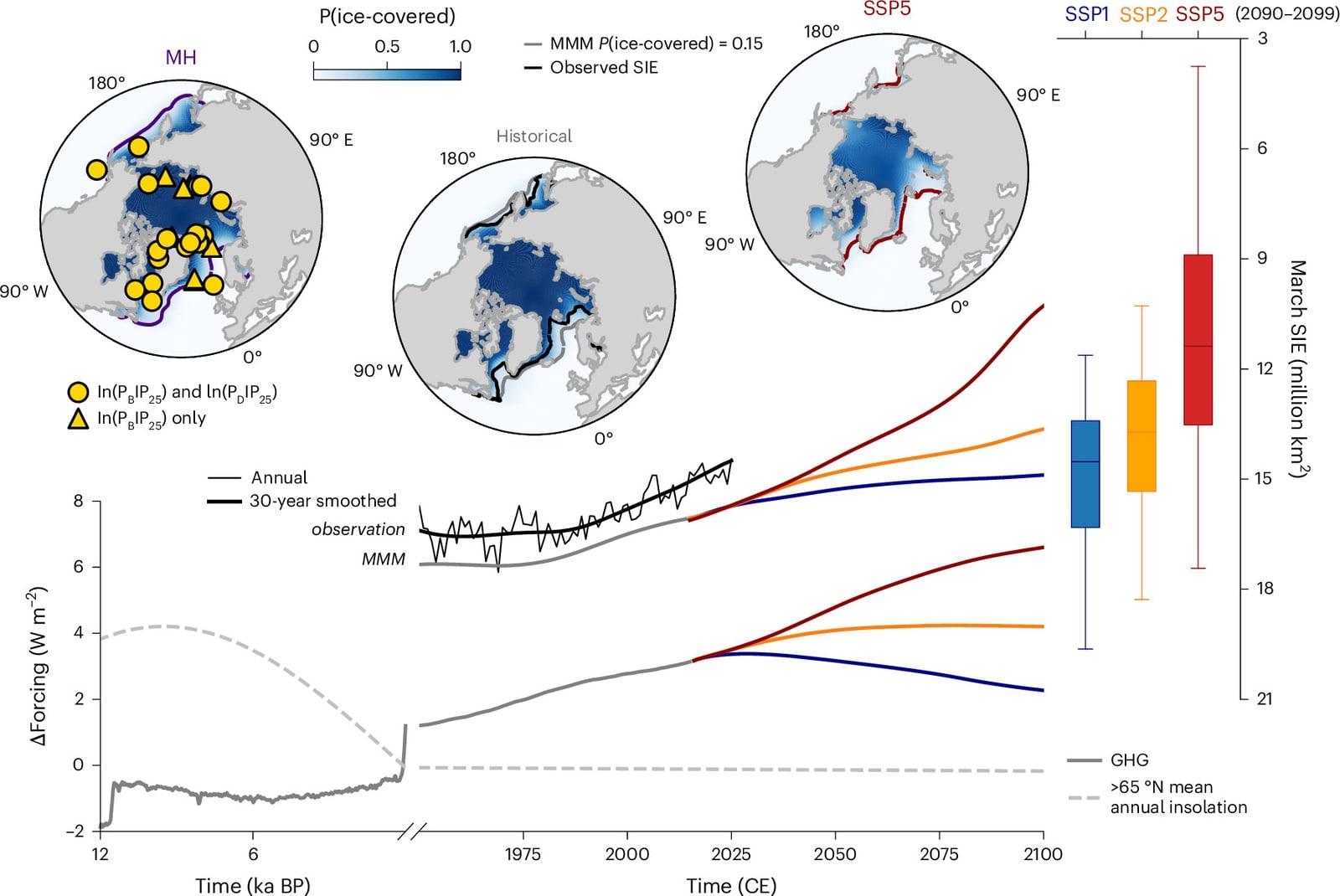
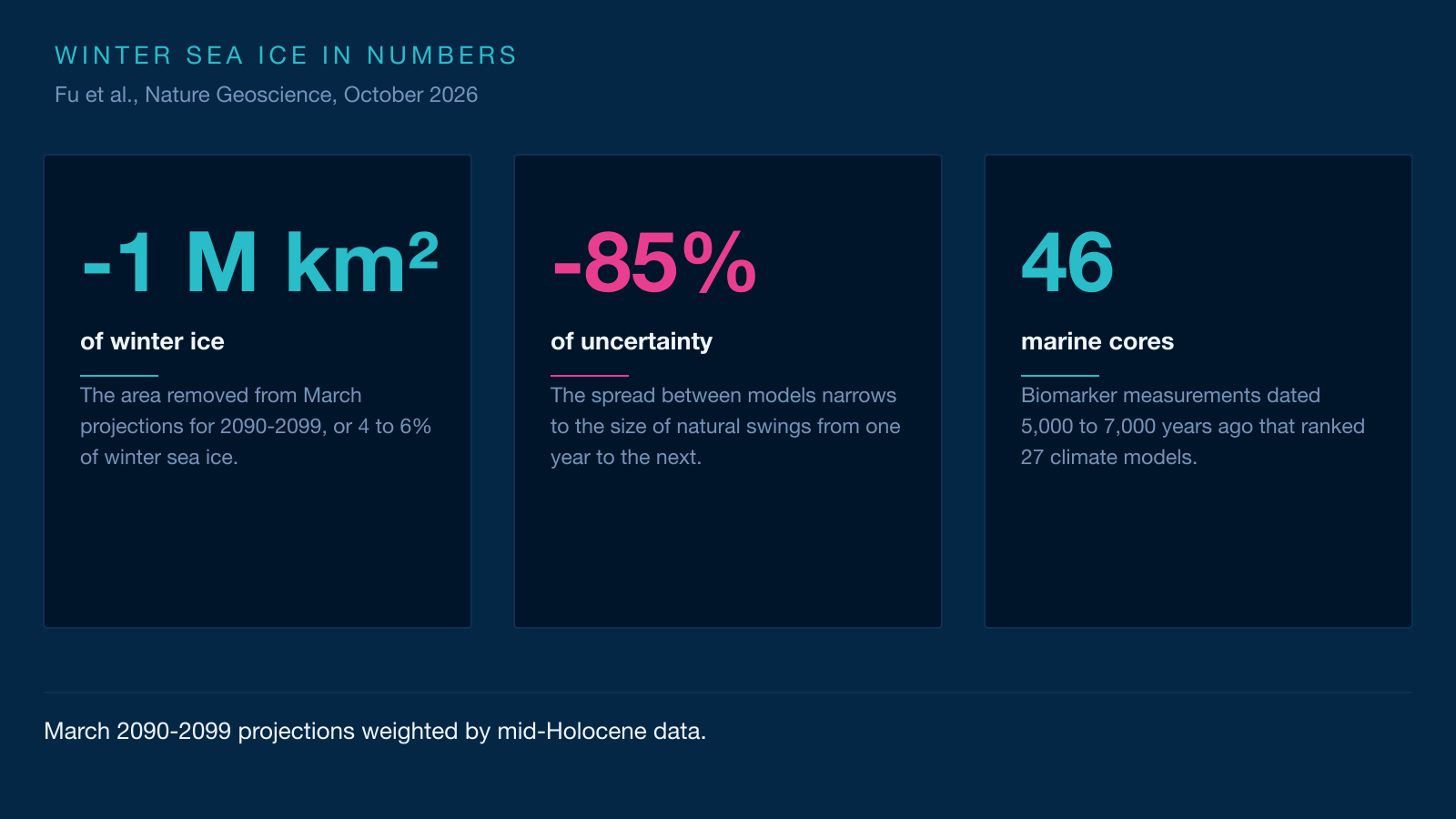
The team compiled 46 such measurements, from cores spread between 54° and 83° north. According to the authors, it is the largest such collection ever assembled for the Arctic. And they focused on one specific period: the mid-Holocene, between 5,000 and 7,000 years ago.
That period was not chosen at random. At the time, the shape of Earth's orbit and the tilt of its axis were not quite what they are today. The Arctic received slightly more summer sunlight, and its annual mean temperature was higher than in pre-industrial times, at a level comparable to what greenhouse gases are preparing for us. Sea ice was scarcer. A natural test bed, at full scale.
Sorting 27 models with a 6,000-year-old judge
Now to use that test bed. Twenty-seven climate models have simulated the same period, within an international comparison framework called PMIP. A climate model, put simply, is a very large program that divides the planet into millions of small boxes and computes, hour after hour, how air, water and ice behave. None is right everywhere, and two well-built models can still disagree about sea ice.
So the researchers set each one an exam. They took every model's output for the warm period, converted it into biomarker values comparable with the measurements, then checked which one matched the 46 cores best. Then came a statistical method called Bayesian, which means revising your judgement as evidence arrives, the way a jury weighs testimony.
Picture a jury of 27 experts telling the same story with variations. The marine cores play the role of physical evidence: they do not say who is right in the abstract, they say which version matches the traces left on the ground. Each model then receives a weight, and the ensemble average stops being an equal vote and becomes a weighted one.
The technical detail that matters is that the weighting accounts for how similar the models are. Two models built in the same laboratory, sharing chunks of code, are not two independent opinions. The method detects this and avoids counting the same testimony twice. Models from the MPI and MIROC groups come out with the heaviest weights, those from the GISS and CSIRO groups with the lightest. The authors stress that these weights are not a measure of intrinsic model quality, but of each model's contribution to bringing the ensemble in line with the data.
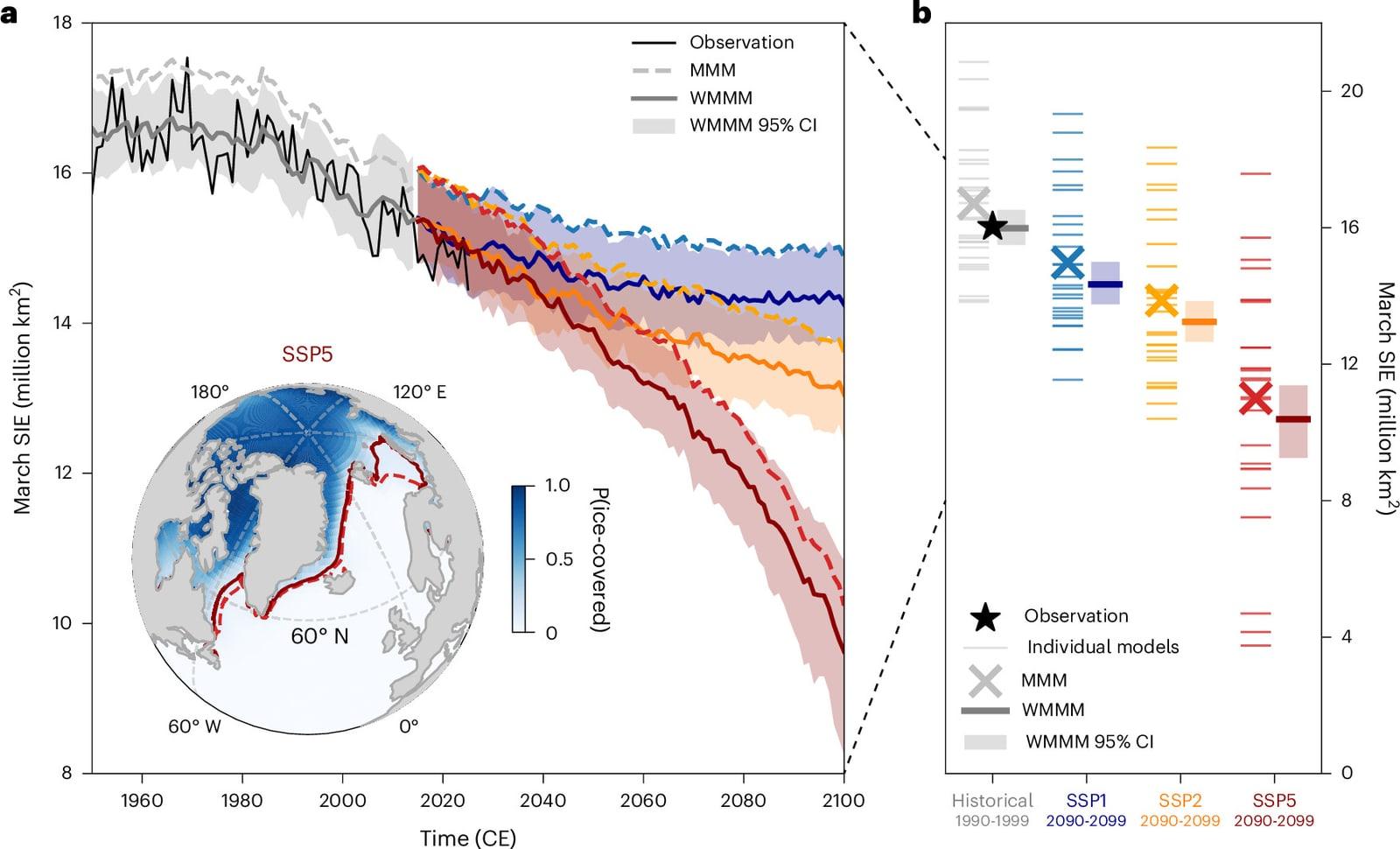
The result is clear-cut. Applied to simulations of the recent past, the weights erase the bias: averaged evenly, the models put too much ice in March. After weighting, the residual drops to 0.016 million km², or 0.099%. And the uncertainty range shrinks by 85%, from a 6.3 million km² spread down to an amplitude comparable with natural year-to-year swings.
A million square kilometres gone, with effects reaching Europe
What follows is straightforward. Since the weights measure how well a model reproduces the sensitivity of sea ice, they can be used to weight its future projections. Same 27 models, same weights, three emissions pathways: a sustainable scenario, a middle-of-the-road one, and a fossil-fuelled one.
In all three cases, the weighted average falls below the plain average. The gap reaches about one million km² over 2090-2099, or 4 to 6% of winter extent. That is a modest percentage and an enormous area: a million square kilometres is close to twice the size of France.
The map shows where it happens. The likeliest losses cluster in the Barents Sea, off eastern Greenland and in the Labrador Sea. The ice edge would shift up to 5.5° of latitude northward, roughly 600 km, the distance from London to Aberdeen. These are also the three regions where recent observations already show the sharpest retreat, which makes the result hang together.
The study goes further and examines two consequences, cautiously. Applying their new weights to precipitation projections, the researchers find that snowfall over southeast Greenland would be underestimated by more than 30% late in the century under the highest-emissions scenario, an extra 44 mm of snow over three months. That snow falls precisely on the ice sheet, where it delays the onset of surface melting.
Another lead, in the Mediterranean. Late-century winter and spring rainfall could reach twice what the plain model average predicts, 92 mm more over the season. That would raise flood risk in southern Europe, though the authors take care to note that these links need confirmation.
This is where the paper leaves pure climatology and touches everyday weather. Less winter sea ice releases more heat and moisture into the atmosphere. That surplus disturbs the polar vortex, the whirl of winds that keeps cold air penned above the Arctic. A weakened vortex lets frigid air spill further south, which can bring cold, snowy winters to the UK, northern Europe and North America.
The link is documented, but it is not mechanical. No two winters are alike, and other factors, such as Atlantic temperatures or stratospheric winds, come into play. The honest phrasing is the authors' own: the odds of those cold, wet winters rise, without anyone being able to call a given year in advance.
What this study does not say
Three limits deserve stating, because they are part of the result.
The first is that the warm period 6,000 years ago was not heated by the same cause as today. Back then it came down to orbit and sunlight. Today it is greenhouse gases. The lead author, Crystal Fu of the Scott Polar Research Institute, owns that choice and defends it: "It doesn't matter if the warming is natural variation or caused by human activity: if it warms, sea ice is going to melt." Her argument is that the physics of ice does not change with the reason for the warming.
The second is that the method assumes the sensitivity of sea ice stays the same in the future. That is a reasonable assumption, but an assumption nonetheless. If a new mechanism kicks in, such as the complete loss of multi-year ice, the weighting could lose part of its relevance.
The third is that 46 cores do not cover the whole Arctic. The sampling points cluster near today's ice edge, in the Labrador Sea and around Greenland, where models diverge most. That is both a strength, because those are the most informative sites, and a limit, because the central ocean remains thinly sampled.
One deeper question remains, and the study does not settle it. The disagreement between models does not vanish, it moves. We now know the ensemble runs too icy in winter, and by how much. We still do not know why some models handle ice badly, or what would have to change in their code for them to get it right without statistical correction. That is the next job.
For now, a simple conclusion stands. The winter Arctic will not merely be freer of ice than expected. It will be so by margins that already touch the heat and moisture maps of the northern hemisphere. And the method used here, putting the models of the future through an exam set by the past, works for other variables besides sea ice. Climate can also be judged on what it has already written down.
Going further
- Track the planet from orbit: our live Earth page gathers the indicators measured by satellite, and the observing guide explains what you are looking at.
- Useful concepts: the atmosphere, which carries the heat and moisture released by the ocean, and Earth's orbit, whose shape explains the climate 6,000 years ago.
- Another climate story, seen from orbit: our article on El Niño 2026 and the satellites measuring it.
- Earth observation does not only come from dedicated satellites. The International Space Station carries downward-pointing instruments such as ECOSTRESS, which measures surface temperature and plant evaporation.
- Sources for this article: the full open-access study in Nature Geoscience, the University of Cambridge release, NASA's page on the March 2026 maximum, the NSIDC data and NOAA's annual Arctic report.