The Global Carbon Budget 2026, a preprint published on 10 November 2026 in Earth System Science Data, projects that global fossil CO2 emissions will fall 0.4% in 2026, to 38.2 GtCO2 (gigatonnes of carbon dioxide, or billion tonnes of the gas). That would be the first decline since 2020 with no crisis attached, and it would place the peak of fossil emissions in 2025. Total emissions are still climbing, and the report also opens up the measurement itself, from a volcano in Hawaii to satellites reading the gas in orbit.
The first drop that is not a crisis
The headline number is small. Global fossil CO2 emissions are projected to fall 0.4% in 2026 against 2025, with a range from a 1.5% drop to a 0.6% rise. In absolute terms that is 10.4 GtC (gigatonnes of carbon) per year, or 38.2 GtCO2, where a tonne of carbon counts as 3.664 tonnes of the gas.
A fraction of a percent is easy to shrug off. The context is not. Emissions grew 1.2% in 2025, to 38.4 ± 1.8 GtCO2. One earlier drop came with a shock, the COVID-19 pandemic of 2020. The 2026 decline would come with none, and 2025 would be the year emissions peaked.
The national figures are uneven. The report projects falls of 0.9% in China, 1.3% in the United States, 1.5% in the European Union and 1.0% in Japan. India runs the other way, with a 4.4% rise, though that number refers to 2025, a year behind the rest.
The carbon intensity of energy, meaning the CO2 released per unit of energy produced, has fallen 0.4% a year for a decade. Forty countries cut fossil emissions while their economies grew between 2016 and 2025, against 22 in the decade before, and those 40 hold 26% of world fossil emissions, or 10.1 GtCO2.
A fossil peak is not a peak in CO2
The trap is in the headline. Fossil fuel is only part of what humans release. Add land-use change, the CO2 that escapes when forest is cleared or drained peat burns, and the 2026 total reaches 43.3 GtCO2, a preliminary estimate, after 42.8 ± 3.2 GtCO2 in 2025. The fossil share falls while the land share rises. Net land-use emissions are put at about 1.4 GtC for 2026, or 5.1 GtCO2, and that climb cancels the fossil dip.
The atmosphere records the sum of both, plus everything emitted before. CO2 concentration is set to reach 427.7 ppm in 2026, 53% above the pre-industrial level of roughly 278 ppm in 1750. A part per million is one molecule of the gas among a million molecules of air, and because the atmosphere has a known mass, 1 ppm of CO2 is 2.124 GtC.
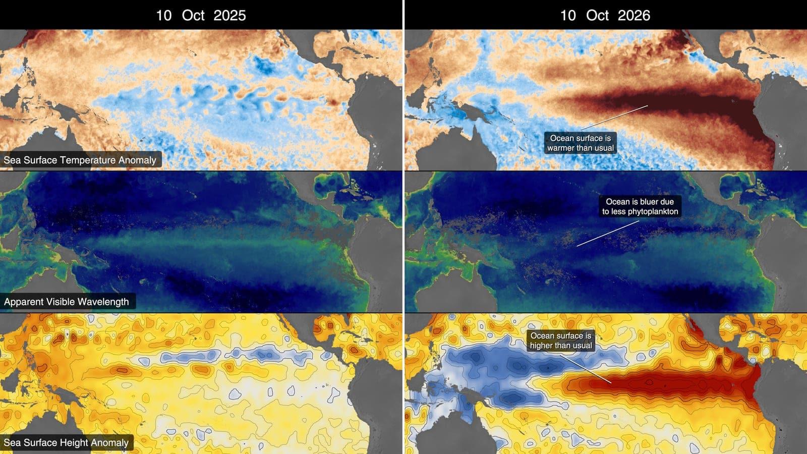
In 2025 the atmosphere gained 4.4 ± 0.2 GtC, or 2.06 ppm, far below the 8.0 ± 0.2 GtC and 3.8 ppm of 2024, largely because the land sink recovered after El Niño. Human activity has already raised the mean temperature 1.37 °C above the pre-industrial baseline.
From the start of 2027, a 50% chance of holding warming to 1.5 °C leaves 40 GtC, or 150 GtCO2, less than four years at the 2026 rate. For 1.7 °C the budget is 510 GtCO2, about 12 years, and for 2 °C it is 1,035 GtCO2, about 24 years.
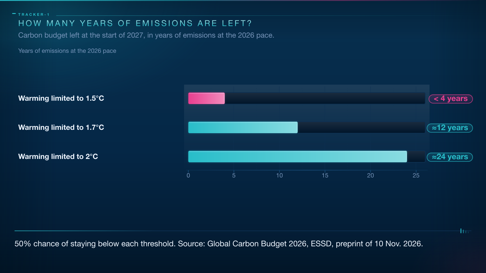
Read that way, 0.4% a year is not fast enough. Stopping the rise is a first step. Making the total fall is the step that counts.
How scientists count a gas they cannot see
The budget is a balance sheet with three entries. Every tonne of CO2 humans release lands in the atmosphere, in the ocean or on land, and each term comes from a different method.
The fossil term is the least direct. It is built from inventories of energy use and cement manufacture, multiplied by emission factors: the carbon each fuel releases per unit burned. No satellite watches a power station plume and adds up the fuel. Fuel statistics are the measurement.
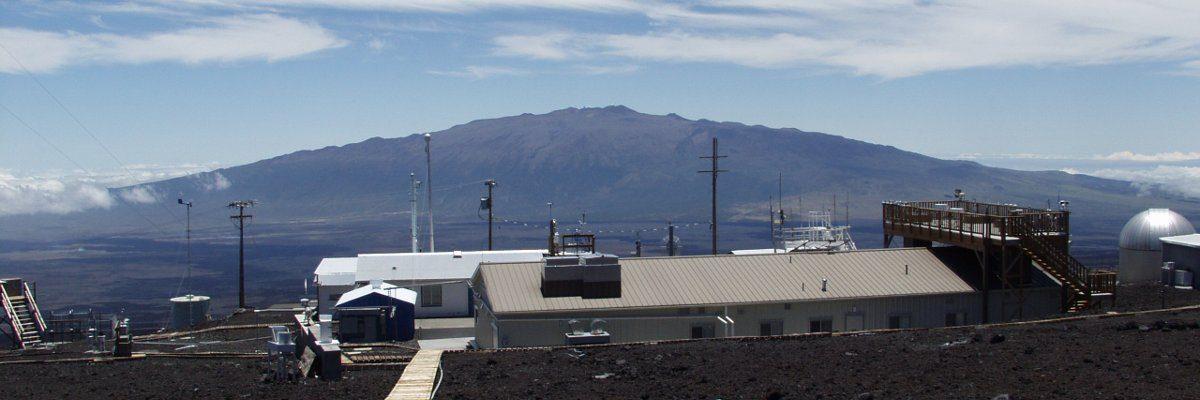
The atmospheric term is the most direct, and it has one address. At Mauna Loa, in Hawaii, C. David Keeling of the Scripps Institution of Oceanography started continuous readings in March 1958. The station measures at 3,400 m on a Pacific volcano, above the local air, so the air it samples has been stirred by winds for days and stands for a large slice of the hemisphere. The record shows a sawtooth: a yearly rise plus the breathing of Northern Hemisphere forests each spring. In September 2026 the station read 426.07 ppm, against 424.37 ppm a year earlier.
The ocean and land terms are modelled. Ocean uptake comes from biogeochemistry models and surface CO2 pressure measurements, land uptake from dynamic vegetation models, programs that grow and kill plants and track soil carbon.
Before any number can be added, readings are scaled to the 2019 calibration scale of the World Meteorological Organization, the WMO.
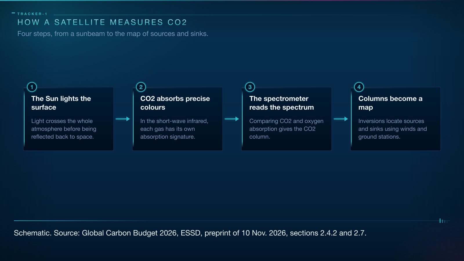
The last step is where satellites enter. An atmospheric inversion runs the arithmetic backwards, from measured concentrations and known winds to the emissions that would produce them, the way you locate a fire in a windowless building from the smell in each room.
What a satellite sees when it looks at CO2
The measurement starts with the Sun. No laser is fired at the ground. Sunlight reflected by the surface crosses the whole atmosphere on its way up, and along the way CO2 absorbs part of it. In the short-wave infrared, a band just beyond the red the eye can see, CO2 carves a pattern of specific colours out of the spectrum, like narrow notches cut in a rainbow. Oxygen carves its own, at known wavelengths.
A spectrometer reads that pattern. It is a prism with a detector: a grating spreads light into its colours and the detector measures how much of each survives. Comparing the CO2 notches with the oxygen notches cancels the effects of surface brightness and sunlight angle.
The result is XCO2, the column-averaged dry-air mole fraction of CO2. Column-averaged: one number for the whole column, ground gas and high-altitude gas merged. Dry air: water vapour is removed, so humidity does not blur the carbon signal. Mole fraction: a share of molecules rather than a mass, which is why the answer comes in ppm.
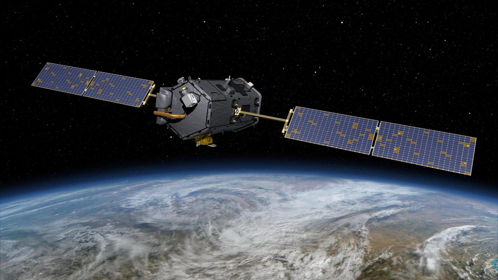
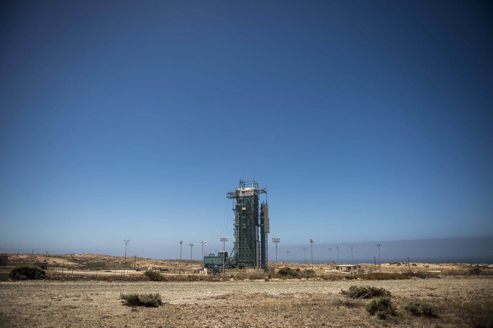
The ground patch under each measurement, its footprint, varies by satellite. GOSAT, in orbit since 23 January 2009, averages 80 km² per sounding and revisits almost the whole globe every three days. OCO-2, launched on 2 July 2014, resolves 3 km² and gives daily global coverage, fine enough to follow carbon between reservoirs and watch vegetation.
OCO-3 went up on 3 May 2019 and works from the International Space Station, taking targeted looks at cities and ecosystems at different hours, which shows how plant activity changes through the day.
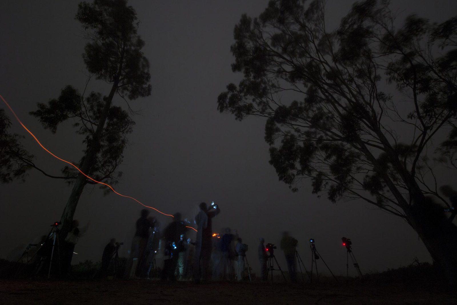
MicroCarb, launched by CNES in the night of 25 to 26 July 2025, maps sources and sinks with a grating spectrometer good to about 1 ppm at 4.5 km by 9 km. CO2M, the European constellation built by ESA and run by EUMETSAT for Copernicus, will fly three satellites, the first due at the end of 2027, built for at least 7.5 years of operation. Its CO2 and NO2 imaging spectrometer works at 4 km², and a multi-angle polarimeter and a cloud imager correct for aerosols and clouds.
The column is not a straight sum of the whole atmosphere: sensitivity to CO2 in the surface layer, where emissions are released, is far higher than to gas high in the stratosphere. A satellite is at its best where the story happens.
What the satellites add, and what they cannot do
Satellites have earned their place. Of 16 inversion systems in the report, 11 use XCO2 from GOSAT or OCO-2, and five add the columns to ground records rather than swap them out.
The numbers support the method. The satellite-derived growth rate known as GRESO reached 4.2 ± 0.2 GtC in 2025, or 1.96 ppm, against 4.4 ± 0.2 GtC and 2.06 ppm from surface stations. Both routes land within their uncertainties, and their year-to-year swings match at a correlation of 0.91.
The limits are real. Clouds block the view, aerosols scatter light in ways that mimic absorption, and the average blends a plume with the clean air beside it. Above all, a satellite cannot tell fossil carbon from the breath of a forest alone. The workaround comes from winds, from models and soon from a second gas: the NO2 channel on CO2M exists because nitrogen dioxide is a short-lived marker of combustion.
None of this retires the ground network. Over the past decade the ocean took up 27% of emissions and the land 22%, and warming is shrinking both, cutting the ocean sink by 8% and the land sink by 19% over 2016-2025. The land sink swung from 2.5 ± 0.8 GtC a year to 3.6 in 2025 and 4.1 in 2026 as it recovered. The ocean sink held at 3.0 ± 0.6 GtC a year, at 3.1 GtC in 2026, and has stayed flat since 2016. A flat sink facing rising emissions is the arithmetic under it.
Going further
- Follow the planet from orbit: our live Earth page collects satellite indicators, and the observing guide decodes them.
- The tools behind the record: spectroscopy, which reads a gas in the light it absorbs, the spectrometer that splits that light, the atmosphere that stores the result, and Earth orbit, where the satellites travel.
- Not every CO2 sensor sits on a dedicated satellite. The International Space Station carries OCO-3, which looks down on cities and plant health through the day.
- Sources: the Global Carbon Budget 2026 preprint on ESSD, the NOAA Global Monitoring Laboratory page on Mauna Loa, the NASA OCO-2 mission page, the NASA OCO-3 mission page, the JAXA GOSAT project page, the CNES MicroCarb page and the EUMETSAT CO2M page.